Welcome to pyHaiCS!¶

Introducing pyHaiCS, a Python library for Hamiltonian-based Monte-Carlo methods tailored towards practical applications in computational statistics. From sampling complex probability distributions, to approximating complex integrals, pyHaiCS is designed to be fast, flexible, and easy to use, with a focus on providing a user-friendly interface for researchers and practitioners while also offering users a variety of advanced features.

Although currently still in development, our library implements a wide range of sampling algorithms — including single-chain and multi-chain Hamiltoninan Monte-Carlo (HMC) and Generalized HMC (GHMC); a variety of numerical schemes for the integration of the simulated Hamiltonian dynamics (including a generalized version of Multi-Stage Splitting integrators), or a novel adaptive algorithm — Adaptive Integration Approach in Computational Statistics (s-AIA) — for the automatic tuning of the parameters of both the numerical integrator and the sampler.

Likewise, several utilities for diagnosing the convergence and efficiency of the sampling process, as well as multidisciplinary benchmarks — ranging from simple toy problems such as sampling from specific distributions, to more complex real-world applications in the fields of computational biology, Bayesian modeling, or physics — are provided.

pyHaiCS Features¶

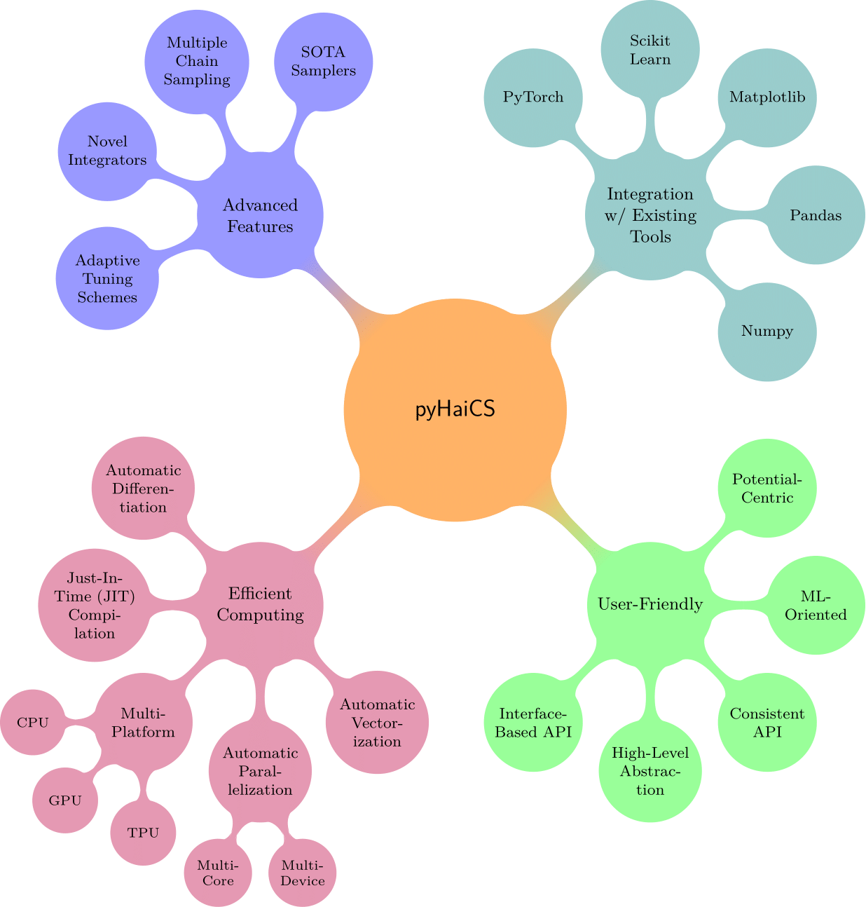
The main features of pyHaiCS, as summarized in the figure below, include its:

Efficient Implementation: pyHaiCS is built on top of the JAX library developed by Google which provides automatic differentiation for computing gradients and Hessians, and Just-In-Time (JIT) compilation for fast numerical computations. Additionally, the library is designed to take advantage of multi-core CPUs, GPUs, or even TPUs for accelerated sampling, and to be highly parallelizable (e.g., by running each chain of multi-chain HMC in a separate CPU core/thread in the GPU).
User-Friendly Interface: The library is designed to be easy to use, with a simple and intuitive API that abstracts away the complexities of Hamiltonian Monte-Carlo (HMC) and related algorithms. Users can define their own potential functions and priors, and run sampling algorithms with just a few lines of code.
Integration with Existing Tools: The library is designed to be easily integrated with other Python libraries, such as NumPy, SciPy, and Scikit-Learn. This allows users to leverage existing tools and workflows, and build on top of the rich ecosystem of scientific computing in Python. Therefore, users can easily incorporate pyHaiCS into their existing Machine Learning workflows, and use it for tasks such as inference, model selection, or parameter estimation in the context of Bayesian modeling.
Advanced Features: pyHaiCS supports a variety of Hamiltonian-inspired sampling algorithms, including single-chain and multi-chain HMC (and GHMC), generalized \(k\)-th stage Multi-Stage Splitting integrators, and adaptive integration schemes (such as s-AIA).

In order to provide a functional and easy-to-use library, and especially to ensure that our code can be easily integrated into existing workflows, we have designed pyHaiCS with a simple rule in mind: Objects are specified by interface, not by inheritance. That is, much alike Scikit-Learn, inheritance is not enforced; and instead, code conventions provide a consistent interface for all samplers, integrators, and utilities. This allows for a more flexible and modular design, and makes it easier for users to extend the library with their own custom implementations. As Scikit's design around making all estimators have a consistent fit and predict interface, pyHaiCS follows a similar approach, but with a focus on Hamiltonian Monte-Carlo methods and its related algorithms. For instance, all integrators in pyHaiCS have a consistent integrate method, which takes as input the potential function, the initial state, and the parameters of the integrator, and returns the final state of the system after the integration process. This consistent interface makes it easy for users to switch between different integrators, or to implement their own custom integrators, without having to worry about the underlying details of the implementation.

Moreover, pyHaiCS is designed to be highly modular, with each component of the library being self-contained and independent of the others, as well as being easily extensible and customizable. As a further point of strength, our library handles all auto-differentiation (such as potential gradients and Hessians) through the JAX library, which provides a fast and efficient way to compute gradients as well as a higher level of abstraction for the user to focus on the actual problem at hand. By only defining the potential function of the Hamiltonian, the user can easily run the sampler and obtain the posterior distribution of the parameters of interest. As an example of the ease-of-use of pyHaiCS, we show below a simple example of how to define a Bayesian Logistic Regression (BLR) model:

# Step 1 - Define the BLR model
@jax.jit
def model_fn(x, params):
    return jax.nn.sigmoid(jnp.matmul(x, params))

# Step 2 - Define the log-prior and log-likelihood
@jax.jit
def log_prior_fn(params):
    return jnp.sum(jax.scipy.stats.norm.logpdf(params))

@jax.jit
def log_likelihood_fn(x, y, params):
    preds = model_fn(x, params)
    return jnp.sum(y * jnp.log(preds) + (1 - y) * jnp.log(1 - preds))

# Step 3 - Define the log-posterior (remember, the oppositve of the potential)
@jax.jit
def log_posterior_fn(x, y, params):
    return log_prior_fn(params) + log_likelihood_fn(x, y, params)

# Initialize the model parameters (including intercept term)
key = jax.random.PRNGKey(42)
mean_vector, cov_mat = jnp.zeros(X_train.shape[1]), jnp.eye(X_train.shape[1])
params = jax.random.multivariate_normal(key, mean_vector, cov_mat)

# HMC for posterior sampling
params_samples = haics.samplers.hamiltonian.HMC(params, 
                            potential_args = (X_train, y_train),
                            n_samples = 1000, burn_in = 200, 
                            step_size = 1e-3, n_steps = 100, 
                            potential = neg_log_posterior_fn,  
                            mass_matrix = jnp.eye(X_train.shape[1]), 
                            integrator = haics.integrators.VerletIntegrator(), 
                            RNG_key = key)

# Average across chains
params_samples = jnp.mean(params_samples, axis = 0)

# Make predictions using the samples
preds = jax.vmap(lambda params: model_fn(X_test, params))(params_samples)
mean_preds = jnp.mean(preds, axis = 0)

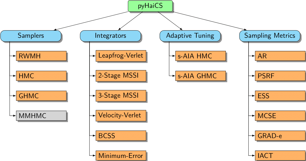
Regarding the actual features implemented in pyHaiCS, and the general organization of its API, the figure below provides a high-level overview of the main components of the library. As can be seen, the library is organized around four main components: Hamiltonian Samplers, Numerical Integrators, Adaptive Tuning, and Sampling Metrics. Each of these components is further divided into sub-components, such as the different samplers implemented in the library (e.g., HMC, GHMC, and the yet to be implemented, MMHMC), the numerical integrators (such as variants of Velocity-Verlet, and 2-Stage and 3-Stage MSSIs), or the s-AIA adaptive tuning scheme. The library also includes a variety of sampling metrics for diagnosing the convergence and efficiency of the sampling process, as well as multidisciplinary benchmarks (and code examples) for testing the performance of the library.

Introduction to Hamiltonian Monte-Carlo¶

Markov-Chain Monte-Carlo (MCMC) methods are powerful tools for sampling from complex probability distributions, a task that lies at the heart of many statistical and Machine Learning problems. Among these, Hamiltonian Monte-Carlo (HMC) stands out as a particularly efficient and versatile algorithm, especially well-suited for high-dimensional problems.

Traditional MCMC methods, such as the Metropolis-Hastings algorithm or Gibbs sampling, often rely on random walk behavior to explore the target distribution. While effective, this can lead to slow convergence, especially when dealing with complex, multimodal, or high-dimensional distributions. HMC addresses these limitations by introducing concepts from Hamiltonian dynamics to guide the exploration of the sample space.

At its core, HMC leverages the idea of simulating the movement of a particle in a physical system to generate efficient transitions across the target distribution \(\pi(\mathbf{q})\). Let's break down the key elements:

Augmenting the State Space: Imagine the probability distribution we want to sample from – our target distribution – as defining a potential energy landscape. Regions of high probability correspond to valleys (low potential energy), while regions of low probability are hills (high potential energy). To introduce dynamics, HMC augments our state space by adding auxiliary momentum variables, typically denoted as \(\mathbf{p}\), for each position variable \(\mathbf{q}\) (our original parameters of interest).
Hamiltonian Function: We then define a Hamiltonian function, \(H(\mathbf{q}, \mathbf{p})\), which describes the total energy of the system. This function is typically the sum of two components:
- Potential Energy, \(U(\mathbf{q})\): This is directly related to our target probability distribution, \(\pi(\mathbf{q})\). Specifically, we often set \(U(\mathbf{q}) = -\log \pi(\mathbf{q})\). Minimizing the potential energy corresponds to finding regions of high probability under \(\pi(\mathbf{q})\).
- Kinetic Energy, \(K(\mathbf{p})\): This term depends on the momentum variables and is usually defined as the energy of a fictitious "particle" associated with our system. A common choice is the kinetic energy of a particle with unit mass: \(K(\mathbf{p}) = \frac{1}{2} \mathbf{p}^T \mathbf{M}^{-1} \mathbf{p}\), where \(\mathbf{M}\) is a mass matrix (often set to the identity matrix for simplicity).
The Hamiltonian is then \(H(\mathbf{q}, \mathbf{p}) = U(\mathbf{q}) + K(\mathbf{p}) = -\log \pi(\mathbf{q}) + \frac{1}{2} \mathbf{p}^T \mathbf{M}^{-1} \mathbf{p}\).
Hamilton's Equations of Motion: The dynamics of the system are governed by Hamilton's equations of motion. These equations describe how the positions and momenta evolve over time:

\[ \begin{aligned} \frac{d\mathbf{q}}{dt} &= \frac{\partial H}{\partial \mathbf{p}} = \mathbf{M}^{-1} \mathbf{p} \\ \frac{d\mathbf{p}}{dt} &= -\frac{\partial H}{\partial \mathbf{q}} = -\frac{\partial U}{\partial \mathbf{q}} = \nabla \log \pi(\mathbf{q}) \end{aligned} \]

These equations dictate that the "particle" will move through the potential energy landscape. Crucially, under these dynamics, the Hamiltonian \(H(\mathbf{q}, \mathbf{p})\) (and thus the density \(\propto \exp(-H(\mathbf{q}, \mathbf{p}))\)) remains constant over time in a continuous system.
Numerical Integration: To simulate these dynamics on a computer, we need to discretize time and use a numerical integrator. pyHaiCS offers a variety of numerical integrators, including symplectic integrators, which are particularly well-suited for Hamiltonian systems because they preserve important properties of the dynamics, such as volume preservation and near-conservation of energy.
Metropolis Acceptance Step: While the Hamiltonian dynamics ideally preserve the target distribution, numerical integration introduces approximations, and thus trajectories are not perfectly Hamiltonian. To correct for these errors and ensure we are still sampling from the exact target distribution, HMC incorporates a Metropolis acceptance step. After evolving the system for a certain time using numerical integration, we compute the change in Hamiltonian, \(\Delta H\), between the start and end points of the trajectory. We then accept the proposed new state with probability:

\[ \alpha = \min\left(1, \exp(-\Delta H)\right) = \min\left(1, \exp(H(\mathbf{q}_{old}, \mathbf{p}_{old}) - H(\mathbf{q}_{new}, \mathbf{p}_{new}))\right) \]

If the proposal is rejected, we simply retain the previous state. This acceptance step guarantees that the HMC algorithm samples from the correct target distribution, even with numerical integration approximations.

Benefits of HMC:

By leveraging Hamiltonian dynamics, HMC offers several advantages over traditional MCMC methods:

Efficient Exploration of State Space: The Hamiltonian dynamics allows for more directed and less random-walk-like exploration of the target distribution. Trajectories tend to follow gradients of the potential energy, enabling the sampler to move more quickly across the state space, especially in high dimensions.
Reduced Random Walk Behavior: Unlike algorithms relying on random proposals, HMC trajectories can travel significant distances in state space in each step, leading to faster convergence and more efficient sampling, particularly for distributions with complex geometries or long, narrow regions of high probability.
Scalability to High Dimensions: The efficiency gains of HMC become more pronounced as the dimensionality of the problem increases, making it a powerful tool for complex statistical models with many parameters.

In summary, Hamiltonian Monte Carlo provides a robust and efficient approach to MCMC sampling by harnessing the principles of Hamiltonian dynamics. By carefully simulating the physical movement of a system guided by the target distribution, HMC overcomes many limitations of traditional MCMC methods, enabling faster and more reliable sampling from complex, high-dimensional probability distributions. pyHaiCS aims to make these powerful methods accessible and easy to use for a wide range of applications in computational statistics and beyond :)

References

pyHaiCS is an open-source project and is actively maintained and developed by a team of researchers and practitioners in the field of computational statistics. We welcome contributions from the community, and encourage users to report issues, suggest new features, and contribute to the development of the library.
This project was initially conceived as a Python implementation of the work presented in the following publications. However, the library has since evolved into a more general-purpose tool for Hamiltonian-based Monte-Carlo methods in computational statistics and now includes a variety of additional features and functionalities.
- L. Nagar, M. Fernández-Pendás, J. M. Sanz-Serna, E. Akhmatskaya, Adaptive Multi-stage Integration Schemes for Hamiltonian Monte Carlo. Journal of Computational Physics, 502 (2024) 112800. DOI: https://doi.org/10.1016/j.jcp.2024.112800
- T. Radivojevic, E. Akhmatskaya, Modified Hamiltonian Monte Carlo for Bayesian Inference. Statistics and Computing, 30 (2020) 377-404. DOI: https://doi.org/10.1007/s11222-019-09885-x
- T. Radivojevic. Enhancing Sampling in Computational Statistics Using Modified Hamiltonians. PhD thesis, UPV/EHU, Bilbao (Spain), 2016. URI http://hdl.handle.net/20.500.11824/323