Quick Start
In this introduction notebook we provide a simple implementation of a Bayesian Logistic Regression (BLR) model so that users can become familiarized with our library and how to implement their own computational statistics models.
First, we begin by importing pyHaiCS. Also, we can check the version running...
import pyHaiCS as haics
print(f"Running pyHaiCS v.{haics.__version__}")
Example 1 - Bayesian Logistic Regression for Breast Cancer Classification
As a toy example, we implement below a classic BLR classifier for predicting (binary) breast cancer outcomes...
import jax
import jax.numpy as jnp

from sklearn.datasets import load_breast_cancer
from sklearn.model_selection import train_test_split
from sklearn.preprocessing import StandardScaler

# Load the breast cancer dataset
data = load_breast_cancer()
X, y = data.data, data.target

# Split the dataset into training and testing sets
X_train, X_test, y_train, y_test = train_test_split(X, y, test_size=0.2)

# Standardize the data & convert to jax arrays
scaler = StandardScaler()
X_train = jnp.array(scaler.fit_transform(X_train))
X_test = jnp.array(scaler.transform(X_test))

# Add column of ones to the input data (for intercept terms)
X_train = jnp.hstack([X_train, jnp.ones((X_train.shape[0], 1))])
X_test = jnp.hstack([X_test, jnp.ones((X_test.shape[0], 1))])
First, we train a baseline point-estimate logistic regression model...
from sklearn.linear_model import LogisticRegression
from sklearn.metrics import accuracy_score

def baseline_classifier(X_train, y_train, X_test, y_test):
    clf = LogisticRegression(random_state = 42)
    clf.fit(X_train, y_train)
    y_pred = clf.predict(X_test)
    accuracy = accuracy_score(y_test, y_pred)
    print(f"Accuracy (w/ Scikit-Learn Baseline): {accuracy:.3f}\n")

baseline_classifier(X_train, y_train, X_test, y_test)
Now, in order to implement its Bayesian counterpart, we start by writing the model and the Hamiltonian potential (i.e., the negative log-posterior)...
# Bayesian Logistic Regression model (in JAX)
@jax.jit
def model_fn(x, params):
    return jax.nn.sigmoid(jnp.matmul(x, params))

@jax.jit
def prior_fn(params):
    return jax.scipy.stats.norm.pdf(params)

@jax.jit
def log_prior_fn(params):
    return jnp.sum(jax.scipy.stats.norm.logpdf(params))

@jax.jit
def likelihood_fn(x, y, params):
    preds = model_fn(x, params)
    return jnp.prod(preds ** y * (1 - preds) ** (1 - y))

@jax.jit
def log_likelihood_fn(x, y, params):
    epsilon = 1e-7
    preds = model_fn(x, params)
    return jnp.sum(y * jnp.log(preds + epsilon) + (1 - y) * jnp.log(1 - preds + epsilon))

@jax.jit
def posterior_fn(x, y, params):
    return prior_fn(params) * likelihood_fn(x, y, params)

@jax.jit
def log_posterior_fn(x, y, params):
    return log_prior_fn(params) + log_likelihood_fn(x, y, params)

@jax.jit
def neg_posterior_fn(x, y, params):
    return -posterior_fn(x, y, params)

# Define a wrapper function to negate the log posterior
@jax.jit
def neg_log_posterior_fn(x, y, params):
    return -log_posterior_fn(x, y, params)
Then, we can call the HMC sampler in pyHaiCS (and sample from several chains at once) with a very high-level interface...
# Initialize the model parameters (includes intercept term)
key = jax.random.PRNGKey(42)
mean_vector = jnp.zeros(X_train.shape[1])
cov_mat = jnp.eye(X_train.shape[1])
params = jax.random.multivariate_normal(key, mean_vector, cov_mat)

# HMC for posterior sampling
params_samples = haics.samplers.hamiltonian.HMC(params,
                            potential_args = (X_train, y_train),
                            n_samples = 1000, burn_in = 200,
                            step_size = 1e-3, n_steps = 100,
                            potential = neg_log_posterior_fn,
                            mass_matrix = jnp.eye(X_train.shape[1]),
                            integrator = haics.integrators.VerletIntegrator(),
                            RNG_key = 120)

# Average across chains
params_samples = jnp.mean(params_samples, axis = 0)

# Make predictions using the samples
preds = jax.vmap(lambda params: model_fn(X_test, params))(params_samples)
mean_preds = jnp.mean(preds, axis = 0)
mean_preds = mean_preds > 0.5

# Evaluate the model
accuracy = jnp.mean(mean_preds == y_test)
print(f"Accuracy (w/ HMC Sampling): {accuracy}\n")
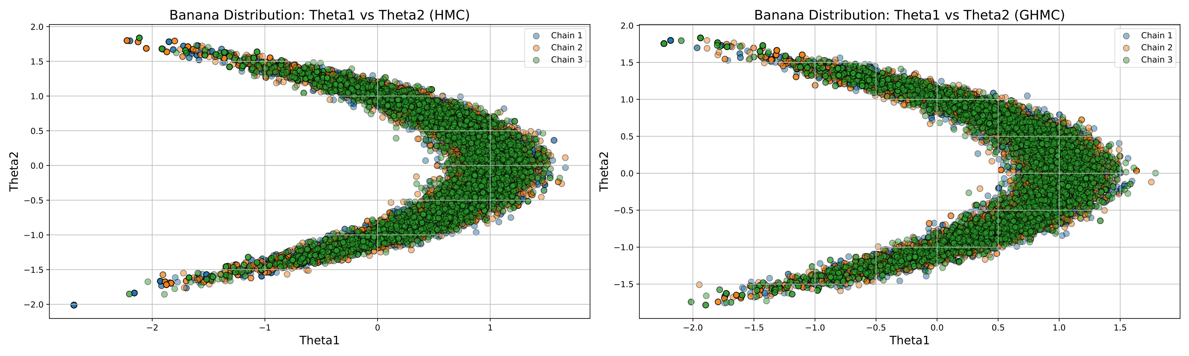
Example 2 - Sampling from a Banana-shaped Distribution
In this example, we will demonstrate how to sample from a banana-shaped distribution using pyHaiCS. This distribution is often used as a benchmark for MCMC algorithms and is defined as follows...
Given data \(\lbrace y_k\rbrace_{k=1}^K\), we sample from the banana-shaped posterior distribution of the parameter \(\symbf{\theta} = (\theta_1, \theta_2)\) for which the likelihood and prior distributions are respectively given as:
The sample data are generated with \(\theta_1+\theta_2^2=1, \sigma_y=2, \sigma_{\theta}=1\). Then, the potential is given by:
The resulting samples were produced for 10 independent chains, each with 5000 burn-in iterations, 5000 samples, \(L=14\) integration steps, a step-size of \(\varepsilon=1/9\), and a momentum noise of \(\phi=0.5\).
First, let's generate some synthetic data based on the description. We set \(\theta_1+\theta_2^2=1\), \(\sigma_y=2\), and \(\sigma_{\theta}=1\). We will generate \(K=100\) data points (provided in the benchmarks), and then estimate the parameter posteriors using HMC or any other sampler.
filePath = os.path.join(os.path.dirname(__file__),
                        f"../pyHaiCS/benchmarks/BNN/Banana_100.txt")
y = pd.read_table(filePath, header = None, sep = '\\s+').values.reshape(-1)

# Initialize the model parameters
key = jax.random.PRNGKey(42)
key_HMC, key_GHMC = jax.random.split(key, 2)
mean_vector = jnp.zeros(2)
cov_mat = jnp.eye(2)
params = jax.random.multivariate_normal(key_HMC, mean_vector, cov_mat)
sigma_y, sigma_params = 2, 1

# HMC Sampling
params_samples_HMC = haics.samplers.hamiltonian.HMC(params,
                            potential_args = (y, sigma_y, sigma_params),
                            n_samples = 5000, burn_in = 5000,
                            step_size = 1/9, n_steps = 14,
                            potential = potential_fn,
                            mass_matrix = jnp.eye(2),
                            integrator = haics.integrators.VerletIntegrator(),
                            RNG_key = 120, n_chains = 10)
@jax.jit
def potential_fn(y, sigma_y, sigma_params, params):
    return 1/(2 * sigma_y ** 2) * jnp.sum((y - params[0] - params[1]**2) ** 2) \
             + 1/(2 * sigma_params ** 2) * (params[0] ** 2 + params[1] ** 2)
The results for the first three chains, using HMC & GHMC, are shown below: